This post provides a brief introduction to bootstrapping and in particular, how it can be used to calculate confidence intervals. It focuses on the simplest and most familiar case of bootstrapping, which is a Monte Carlo based non-parametric method.
Author
Mark Andrews
Published
July 6, 2021
Bootstrapping is any one of a set of inter-related methods for statistical inference that uses a finite sample from a population as a proxy to the population itself. Using a sample as a proxy for the population in order to infer properties about the population is the reason it is called bootstrapping. Bootstrapping was first proposed in Efron (1979).
The most widely used and familiar bootstrapping methods are extremely simple, both conceptually and practically, as we will see. However, there are in fact almost countless different variants of bootstrapping methods, and there are many books solely devoted to describing these methods in detail (see, for example, Efron and Tibshirani 1993; Davison and Hinkley 1997; Chernick 2008). Here, we will describe how bootstrapping can be used to calculate confidence intervals. We will focus on the simplest methods, but these also happen to be the most widely and familiar in practice. As we explain below, the key feature of these methods involves repeatedly resampling from a sample, calculating statistics using these repeated samples, and then using various properties to the distribution of these statistics to calculate confidence intervals.
Background: Estimators, sampling distributions, and confidence intervals
To understand bootstrapped confidence intervals, it helps to clarify some background details and context related to frequentist statistical inference.
Let us assume we have observed \(n\) values \[
y_{1:n} = y_1, y_2 \ldots y_i \ldots y_n,
\] where each \(y_i\) is a value on the real line, i.e. \(y_i \in \mathbb{R}\) for all \(i \in 1\ldots n\). For simplicity, let us also assume that these \(n\) values are drawn independently from some unknown probability distribution over \(\mathbb{R}\), which we will denote by \(f\).
Suppose that we wish to estimate the mean of the probability distribution \(f\), which we will denote by \(\theta\). The obvious estimator of \(\theta\) is the sample mean of \(y_{1:n}\), which we will denote by \(\hat{\theta}\). Of course, the value of the sample mean \(\hat{\theta}\) is not always going to be exactly the same value as the population mean \(\theta\). For every given sample of \(n\) values from \(f\), the sample mean \(\hat{\theta}\) will be slightly different. Sometimes it will be higher, and sometimes lower, than the population mean \(\theta\). The sampling distribution of \(\hat{\theta}\) tells us how much \(\hat{\theta}\) varies across repeated samples of \(n\) values from \(f\). One important property of the sampling distributions is its standard deviation, which is known as the standard error. The standard error is the key to many types of inferential statistical, including the confidence interval. For example, if a sampling distribution is normally distributed, which will be the case in general as \(n \to \infty\), the 95% confidence interval for \(\theta\) is given by \[
\hat{\theta} \pm 1.96 \times \mathrm{se},
\] where \(\mathrm{se}\) is the standard deviation of the sampling distribution of the sample mean \(\hat{\theta}\), and where the 1.96 multiplier is due to the 2.5th an 97.5th percentiles in a normal distribution being 1.96 standard deviations below and above, respectively, the mean. More generally, in this normally distributed sampling distribution case, the \(1-\alpha\) confidence interval is \[
\hat{\theta} \pm z_{1-\alpha/2} \times \mathrm{se},
\] where \(z_{1-\alpha/2}\) is the value below which lies \(1-\alpha/2\) of the mass in a standard normal distribution. This method of calculation of the confidence interval is sometimes known as the standard interval method.
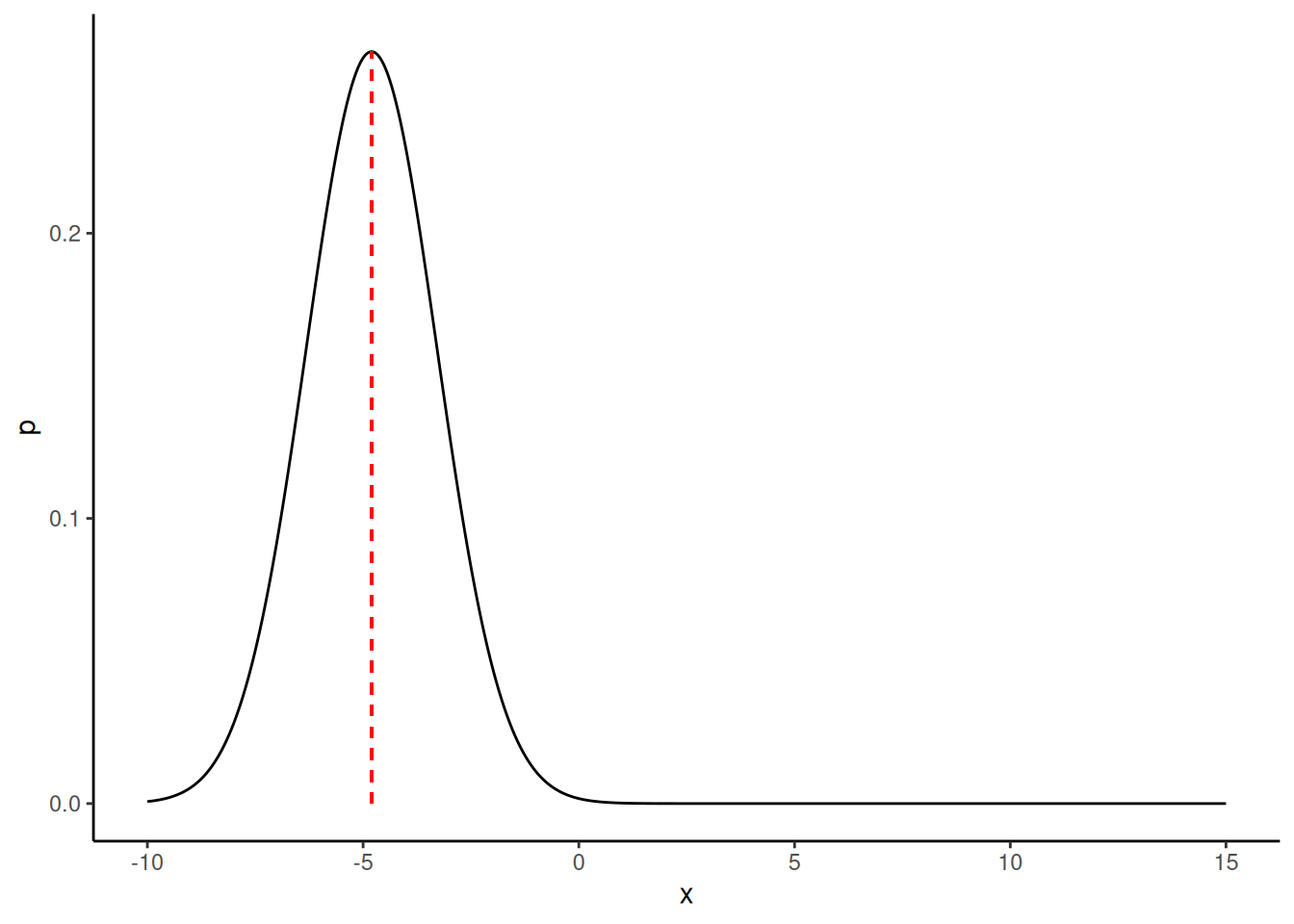
As a concrete illustration of this, let us assume that the probability distribution \(f\) is an exponentially modified Gaussian distribution, also known as an exGaussian distribution. This distribution is roughly like a skewed normal distribution. More precisely, the exGaussian distribution is the distribution of the sum of two independent random variables, one of which is normally distributed, and the other has an exponential distribution. It has three parameters, which we will denoted by \(\mu\), \(\sigma\), and \(\lambda\). These are, respectively, the mean and standard deviation of the normally distributed variable, and the rate parameter of the exponential distribution. A number of R package provide functions for its probability density function, and one such package is emg, where the density function is demg. In the next figure, we plot the density function of the exGaussian when \(\mu = -5\), \(\sigma = 1.5\), and \(\lambda = 5\), and also show the mean of this distribution. This is produced by the following code:
set.seed(10101) # for reproducibilitylibrary(tidyverse)theme_set(theme_classic())mu <--5; vsigma <-1.5; lambda <-5; exgauss_df <-tibble(x =seq(-10, 15, length.out =1000),p = emg::demg(x, mu, vsigma, lambda))# the population meantheta <- mu +1/lambda# density at mean dtheta <- emg::demg(theta, mu, vsigma, lambda)ggplot(exgauss_df,mapping =aes(x = x, y = p)) +geom_line() +geom_segment(x = theta, xend = theta, y =0, yend = dtheta, colour ='red', size =0.5, linetype ='dashed')
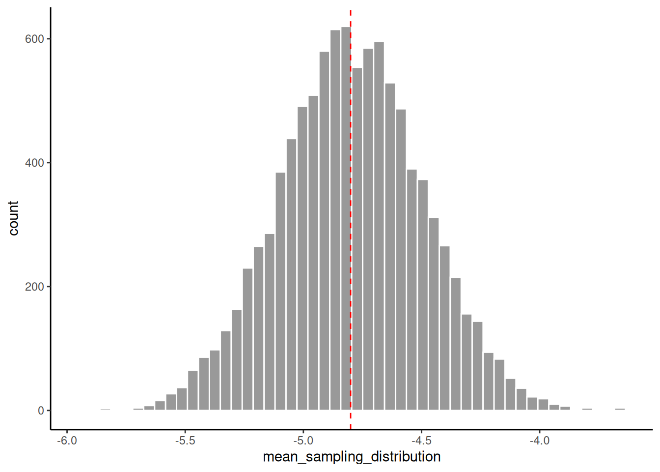
The sampling distribution of the sample mean for the exGaussian with parameters \(\mu = -5\), \(\sigma = 1.5\), \(\lambda = 5\), can be approximated to an arbitrary degree of accuracy by repeatedly sampling \(n\) values from this distribution, and then calculating the sample mean for each sample. The following code repeatedly samples \(n=25\) samples from this exGaussian 10,000 times, and calculates the sample mean in each case.
The standard deviation of this sampling distribution, i.e. the standard error, can be calculated simply by calculating the sample standard deviation of the 10,000 sample means:
se <-sd(mean_sampling_distribution)se
[1] 0.3033802
Now that we know the standard error \(\mathrm{se}\), if we observe a particular sample of size \(n=25\) from the exGaussian with parameters \(\mu = -5\), \(\sigma = 1.5\), \(\lambda = 5\), if we assume that the sampling distribution is approximately normal, the mean of this sample, \(\hat{\theta}\), can be used to give us the approximate 95% confidence interval for \(\theta\) as follows: \[
\hat{\theta} \pm 1.96 \times \mathrm{se}.
\] For example, we can obtain \(n=25\) samples from this exGaussian as follows:
y <- emg::remg(25, mu, vsigma, lambda)
The mean of this sample is
mean(y)
[1] -5.186576
and so the approximate 95% confidence interval based on this sample is \[
(-5.78, -4.59),
\] which we can calculate in R as follows:
mean(y) +c(-1, 1) *1.96* se
[1] -5.781202 -4.591951
Obviously, the procedure we just followed to calculate approximate confidence intervals for \(\theta\) can not be followed in practice. In practice, we do not know the population probability distribution \(f\), so can not numerically calculate the sampling distribution of an estimator like the sample mean. In practice, we can still sometimes rely on theoretical results to estimate the standard error or the sampling distribution generally. For example, if the parameter of interest is the mean of a normal distribution, and the estimator is the sample mean, widely used theoretical results tell us that the standard error is \(\sigma/\sqrt{n}\), where \(\sigma\) is the standard deviation of the normal distribution, which can be approximated by \(s/\sqrt{n}\), where \(s\) is the sample standard deviation. However, theoretical results like this are not always possible. For example, in the case of the exGaussian distribution, or for many other distributions, we do not have an analytic form for the sampling distribution for the sample mean.
Bootstrapping
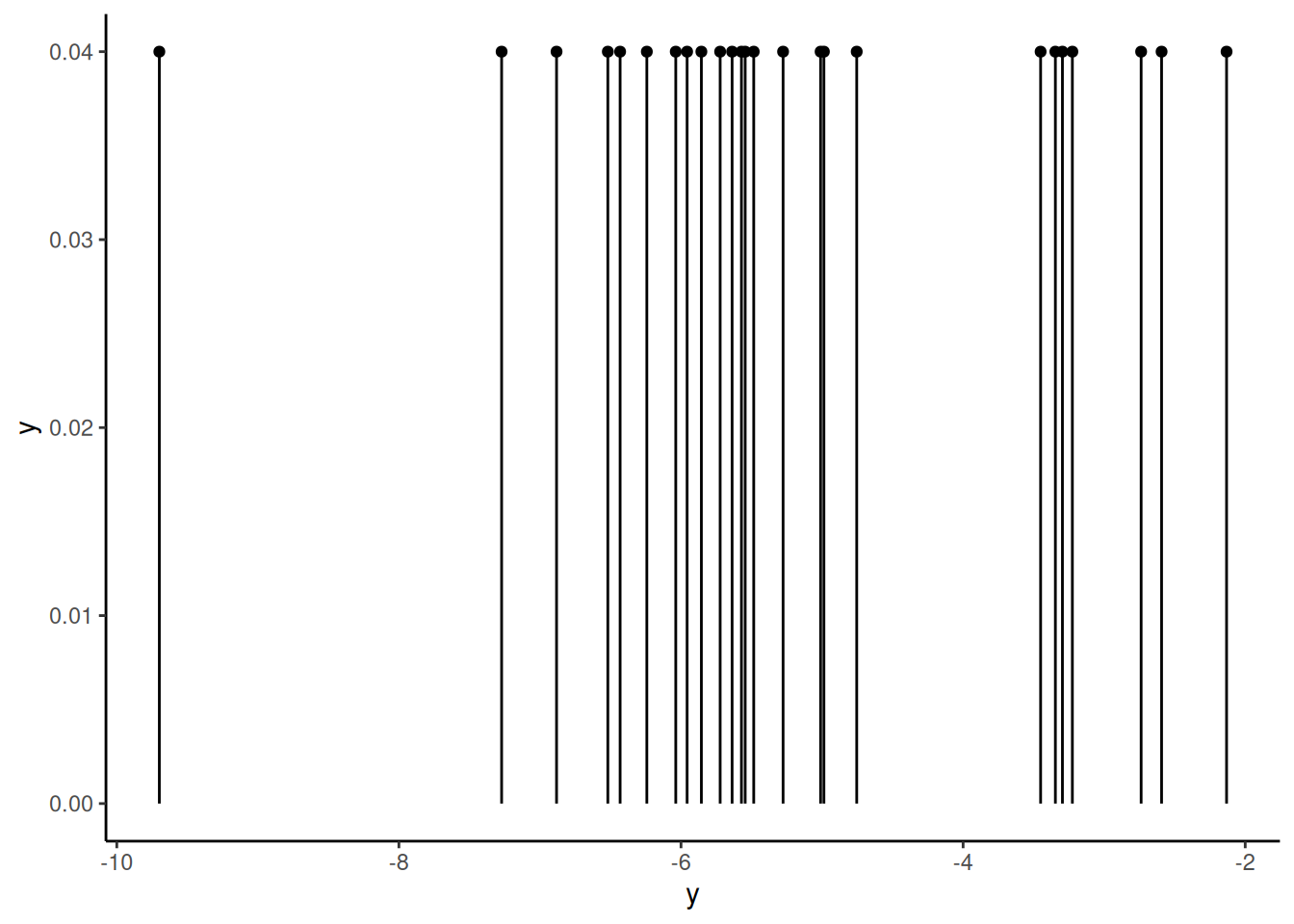
In cases where we do not have analytic form for the sampling distribution of an estimator, we can use bootstrapping. In bootstrapping, we use the empirical distribution of the data, which we will denote \(\hat{f}\), as an approximation to the population distribution \(f\). The empirical distribution is simply the probability distribution of the data itself. In other words, for a sample of \(n\) values, the empirical distribution puts a point-mass of value \(1/n\) at each of the \(n\) values. For the y sample of \(n=25\) values that we obtained above, the plot of the empirical distribution is as follows:
tibble(y, p =1/length(y)) %>%ggplot() +geom_segment(aes(x = y, xend = y, y =0, yend = p)) +geom_point(aes(x = y, y = p))
With \(\hat{f}\) as a our approximation to \(f\), we can now repeatedly sample \(n\) values from \(\hat{f}\), just as we did from \(f\) above, and calculate the sample mean \(\hat{\theta}\) of each sample. This set of values, which we call the bootstrap distribution is then the approximation to the sampling distribution of the sample mean. Sampling \(n\) values from the empirical distribution \(\hat{f}\) is identical to randomly sampling with replacement\(n\) values from the data itself. In R, to randomly sample with replacement \(n = 25\) values from the data vector y, we can simply use the function sample with the replace = TRUE optional argument as follows:
# sample n values, where n is the the length of the vector `y`,# from the empirical distribution of `y`sample(y, replace =TRUE)
We can repeat this sampling 10,000 times, as we did above when we sample from the population distribution, and then calculate the sample mean, as follows:
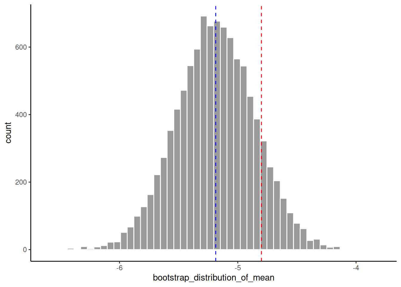
The histogram of this bootstrap distribution is in the next figure, where we also show the population mean \(\theta\) with a vertical red line and the sample mean \(\hat{\theta}\) in a vertical blue line, which is obtained by the following code:
Note how the bootstrap distribution is not centred around \(\theta\), but is centred around \(\hat{\theta}\). This is different to the true sampling distribution above, which is, at least in this example, centered around \(\theta\). This, in fact, turns out to be an important result, as will see below.
We can now use this bootstrap distribution of the estimator \(\hat{\theta}\) to calculate confidence intervals for \(\theta\). There are, in general, many ways to do this, but the two simplest are the standard interval method and the percentile method. The percentile method is arguably the most widely used bootstrapping method of any kind, so much so that it often seen as the definition of bootstrapping in general.
Standard interval method
The standard deviation of the bootstrap distribution, which is our bootstrap based approximation of the standard error, is calculated simply as follows:
As we can see, this is very similar to the confidence interval calculated above where we used the standard deviation of the true, and in general unknown, sampling distribution.
Percentile method
We can, however, also calculate the bootstrap confidence interval just from the percentiles of the bootstrap distribution. This is known as the percentile method for calculating the bootstrap confidence interval (see, for example, Efron and Tibshirani 1993, chap. 13; Efron and Hastie 2016, chap. 11). For example, the 95% bootstrap confidence interval calculated using the percentile method is obtained by finding the 2.5th and 97.5th percentiles of the bootstrap distribution. Using our bootstrap distribution, the percentile method 95% bootstrap confidence is calculated as follows:
Clearly, this is very similar to the previous method that used the bootstrapped standard error.
The percentile method is very simple, and very generally applicable. For any estimator of interest, we can create the bootstrap distribution of this estimator by, as we just demonstrated, repeatedly sampling from the empirical distribution, calculate the estimator for each sample, and the find \(\alpha/2\)th percentile and the \(1-\alpha/2\)th percentile of the bootstrap distribution, which gives us the \(1-\alpha\) bootstrap confidence interval for the parameter that we are estimating.
For example, let us suppose we want confidence intervals for the median, the 10% trimmed mean, the standard deviation, the skewness, or any other parameters or properties of the population, we can proceed by first repeatedly sampling from the empirical distribution \(\hat{f}\):
Note that by specifying simplify = FALSE as an optional argument to replicate, the resulting bootstrap_samples R object is a list with 10,000 elements, each of which is a vector of 25 values. To obtain the 95% confidence interval for the, for example, median, we can use map_dbl to apply the function median to all 10,000 vectors of 25 values, which returns a vector of 10,000 elements, which can then be passed to quantile:
We can perform this calculation for other estimators by replacing the function median with other functions. We can put these functions in a list and iterate over them, passing them to the
The percentile method is, in general, a relatively crude bootstrapping method. Although it is generally better than the standard interval method, there are still many other bootstrapping methods that are more precise (see, for example, Efron 1987; Diciccio and Romano 1988; DiCiccio and Efron 1996). Nonetheless, it is extremely simple, both conceptually and practically. Moreover, in practice, a relatively crude approximation may well be sufficient, and if this can be achieved almost effortlessly in a very wide range of problems, that entails that the method is practically very valuable. It is interesting to consider, therefore, why this very simple method works at all.
Let us begin by assuming for simplicity that the sampling distribution of \(\hat{\theta}\) is normally distributed with a mean of \(\theta\). In other words, we have \[
\hat{\theta} \sim N(\theta, \tau^2),
\] where \(\tau\) is the standard error. As mentioned above, from this we can construct the \(1-\alpha\) confidence interval for \(\theta\) as follows: \[
\hat{\theta} \pm z_{\alpha/2} \times \tau.
\] The values of \(\hat{\theta} + z_{\alpha/2} \tau\) and \(\hat{\theta} - z_{\alpha/2} \tau\) are, respectively, the \(\alpha/2\)th and the \(1-\alpha/2\)th percentiles of the normal distribution centred at \(\hat{\theta}\) and whose standard deviation is \(\tau\). If the bootstrap distribution of \(\hat{\theta}\) is approximately normal and centred at \(\hat{\theta}\) and with a standard deviation of approximately \(\tau\), as was the case with the example above, then the \(\alpha/2\)th and the \(1-\alpha/2\)th percentiles of this distribution will be approximately equal to the confidence interval \(\hat{\theta} + z_{\alpha/2} \times \tau\) and \(\hat{\theta} - z_{\alpha/2} \times \tau\).
In general, we can not assume that the sampling distribution of \(\hat{\theta}\) is normally distributed. However, if there is a invertible function \(g\) such that \(\phi = g(\theta)\) and \(\hat{\phi} = g(\phi)\), and if \(\hat{\phi} \sim N(\phi, \tau_{\phi})\), then \(\hat{\phi} \pm z_{\alpha/2} \times \tau_\phi\) is the \(1-\alpha\) confidence interval on \(\phi\). If the bootstrap of \(\hat{\phi}\) is approximately normal and centred at \(\hat{\phi}\) and with a standard deviation of approximately \(\tau_\phi\), then the \(\alpha/2\)th and the \(1-\alpha/2\)th percentiles of this distribution, which we will denote by \(\hat{\phi}_{\alpha/2}\) and \(\hat{\phi}_{1-\alpha/2}\), respectively, will be approximately equal to the \(1-\alpha\) confidence interval on \(\phi\). If, by the definition of the confidence interval, \(P(\hat{\phi}_{\alpha/2} \leq \phi \leq \hat{\phi}_{1-\alpha/2}) = 1-\alpha\) then \(P(m^{-1}(\hat{\phi}_{\alpha/2}) \leq m^{-1}(\phi) \leq m^{-1}(\hat{\phi}_{1-\alpha/2})) = 1-\alpha\), and \(m^{-1}(\hat{\phi}_{\alpha/2})\) and \(m^{-1}(\hat{\phi}_{1-\alpha/2})\) are the \(\alpha/2\)th and the \(1-\alpha/2\)th percentiles of the bootstrap distribution of \(\hat{\theta} = m^{-1}(\hat{\phi})\).
This means that we do not need to know the function \(m\), we just need to assume that \(m\) exists, or exists approximately. In other words, if we know or can assume that some function \(m\) exists such that \(m(\hat{\theta})\) is normally distributed, or approximately normally distributed, around \(m(\theta)\), then the \(\alpha/2\)th and the \(1-\alpha/2\)th percentiles of the bootstrap distribution of \(\hat{\theta}\) will provide the approximate \(1-\alpha\) confidence interval for \(\theta\).
Bootstrapping in practice in R
In the examples above with used a combination of replicate and sample to make our bootstrap samples. This is already very simple, but there are other functions in various packages in R that can make things even easier. One such function is bootstrap in the modelr package. This is especially useful with working with data frames. The modelr package is part of the tidyverse package collection, so when tidyverse is installed, so too is modelr. It is not loaded automatically when we do library(tidyverse), so we must load it explicitly in the usual manner:
library(modelr)
The modelr::bootstrap function can be used to bootstrap sample a data frame. For example, if we want to draw 10 bootstrap samples from the cars data set, we could do the following:
bootstrap(cars, n =10)
# A tibble: 10 × 2
   strap               .id
   <list>              <chr>
 1 <resample [50 x 2]> 01
 2 <resample [50 x 2]> 02
 3 <resample [50 x 2]> 03
 4 <resample [50 x 2]> 04
 5 <resample [50 x 2]> 05
 6 <resample [50 x 2]> 06
 7 <resample [50 x 2]> 07
 8 <resample [50 x 2]> 08
 9 <resample [50 x 2]> 09
10 <resample [50 x 2]> 10
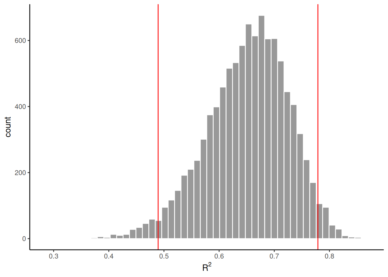
A tibble is returned with a list column named strap. Each element of this column is a single bootstrap sample from cars. We can iterate over the elements of the strap column in many ways, but perhaps the easiest, at least the easiest tidyverse way, is to use the map functional from purrr, which we also used in some examples above. For example, if wanted to calculate bootstrap confidence intervals for \(R^2\) in a linear model predicting dist from speed, we would execute lm(dist ~ speed) for each bootstrap sample and then extract the \(R^2\) value from that model. This could be done as follows, where we use 10,000 bootstrap samples:
get_rsq <-function(m) summary(m)$r.sqboot_rsq <-bootstrap(cars, n =10000) %>% {map_dbl(.$strap,~lm(dist ~ speed, data = .) %>%get_rsq() ) }
The histogram of this bootstrap distribution, where we show the lower and upper bound of the confidence interval is in the next figure, which can be produced by the following code.
Given that we might like to obtain the bootstrap distribution for many different quantities in any lm model, we can make a function that takes an lm model and evaluates it using bootstrap samples from its data:
bootstrap_lm <-function(model, n =10000){ boot <-bootstrap(model$model, n)map(boot$strap, ~lm(formula(model), data = .))}
In this, we rely on the fact that the data used in an lm model is available using the model attribute of the lm object. Likewise, the formula used in the lm model is available using the function formula applies to the lm object. Thus, we too obtain bootstrapped versions from any lm model, we can do the following for example:
M <-lm(dist ~ speed, data = cars)bootstrapped_M <-bootstrap_lm(M)
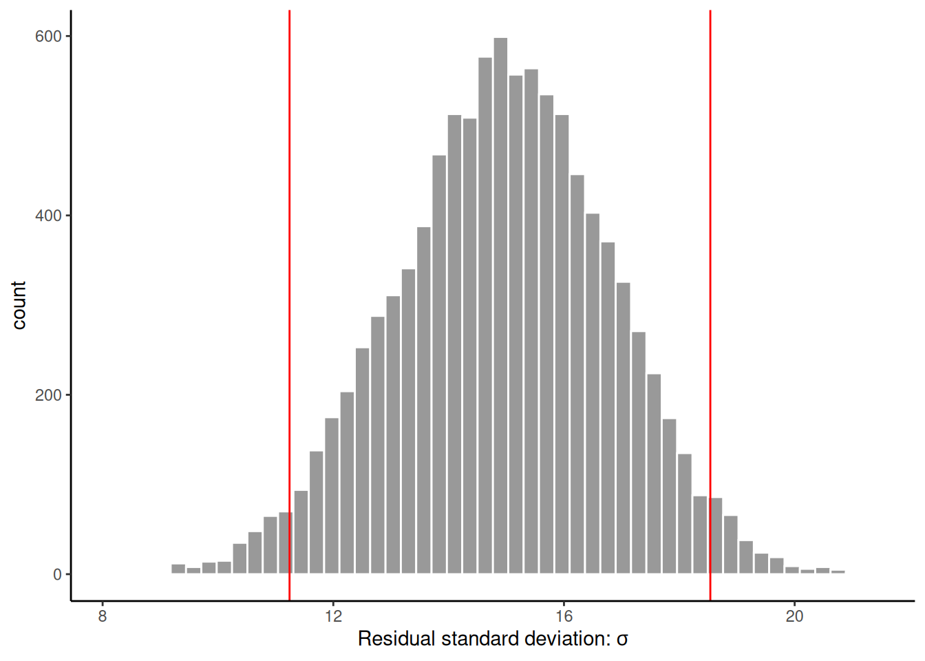
With this, using purrr::map and related functional, we can calculate the bootstrap distribution of any function. For example, we wanted the bootstrap distribution of the residual standard deviation, we could do the following, which uses the sigma function for extracting the residual standard deviation from an lm model.
We can then also use bootstrapped_M to calculate the bootstrap confidence intervals for any set of functions in a list. As an example, in the following code, we calculate the bootstrap confidence intervals for the residual standard deviation, \(R^2\), adjusted \(R^2\), and the AIC:
Chernick, Michael R. 2008. Bootstrap Methods: A Guide for Practitioners and Researchers. John Wiley & Sons.
Davison, Anthony Christopher, and David Victor Hinkley. 1997. Bootstrap Methods and Their Application. 1. Cambridge university press.
DiCiccio, Thomas J., and Bradley Efron. 1996. “Bootstrap Confidence Intervals.”Statistical Science 11 (3): 189–212.
Diciccio, Thomas J, and Joseph P Romano. 1988. “A Review of Bootstrap Confidence Intervals.”Journal of the Royal Statistical Society: Series B (Methodological) 50 (3): 338–54.
Efron, Bradley. 1979. “Bootstrap Methods: Another Look at the Jackknife.”The Annals of Statistics 7 (1): 1–26.
———. 1987. “Better Bootstrap Confidence Intervals.”Journal of the American Statistical Association 82 (397): 171–85.
Efron, Bradley, and Trevor Hastie. 2016. Computer Age Statistical Inference. Cambridge University Press.
Efron, Bradley, and Robert J Tibshirani. 1993. An Introduction to the Bootstrap. Chapman & Hall.