library(parallel)Parallel computing in R with the parallel package
parallel processing
R
This post describes how to do parallel processing in R using the parallel package. First, we will provide a brief general introduction to the parallel programming tools in R’s parallel package. Then, we will explore these tools by way of two applications: bootstrapping, and the parallel execution of Stan based Bayesian models.
Parallel processing is whenever we simultaneously execute multiple programs in order perform some task. To do this, we need two or more computing units (processing units) on our computer. In general, these units can be either cores on the central processing unit (CPU) or on the graphics processing unit (GPU). Modern supercomputing and high performance computing generally almost always uses a mixture of both CPUs and GPUs. However, although most modern desktops and laptop machines usually now have multicore CPUs, most do not have general purpose GPUs, and so we will not consider GPU computing here.
The topic of parallel computing generally is a highly technical one, often focusing on relatively low level programming concepts, the details of the hardware, and the algorithmic details of the task be carried out. Here, we will avoid all of this complexity. We will focus exclusively on what are called embarrassingly parallel problems. These are computing problems can be easily broken down into multiple independent parts. We will also assume that we are working on a single computer (i.e., node), such as a laptop or desktop machine, rather than on a cluster of multiple nodes. And we will focus on parallel computing using R itself, as opposed to the parallelism that we can obtain using libraries such as OpenMP (Open Multi-Processing) or MPI (Message Passing Interface) when programming with C/C++ and other fast level languages.
First, we will provide a brief general introduction to the parallel programming tools in R’s parallel package. Then, we will explore these tools by way of two applications: bootstrapping, and the parallel execution of Stan based Bayesian models.
The parallel package
R provides many packages related to parallel computing. See the webpage https://cran.r-project.org/web/views/HighPerformanceComputing.html for a curated list of relevant packages. Here, we will focus exclusively on the R parallel package. This package builds upon and incorporates two other packages: multicore and snow (simple network of workstations). The principal way that parallel processing is done using parallel is by using multiple new processes that are started by a command in R. These processes are known as workers and the R session that starts them is known as the master. The communication between the master and the workers can be done using sockets, and the code for doing this was developed by snow, or else by forks, and the code for this was developed by multicore. Forks create copies of the master process, including all its objects, and workers and the master processes share memory allocations Sockets are independent processes to which information from and to the master must be explicitly copied. In both forks and sockets, tasks are farmed out to the workers from the master using parallel version of “map” functionals, e.g. lapply, purrr::map, which are described in this blog post. While there are many advantages to using forks, their key disadvantage is that they are not available on Windows. For that reason, we will only consider sockets here.
The parallel package is pre-installed in R and is loaded with the usual library command.
We can use the detectCores function from parallel to list the number of available cores on our computer. The option logical = FALSE will list only physical, rather than virtual, cores. It is advisable to always set logical = FALSE and so report only physical cores as this in general list the maximum number of separate processes that can be executed simultaneously. The machine on which I am currently working is a AMD Ryzen 7 3700X 8-Core Processor, and so there are 8 physical cores
Using clusterCall, clusterEvalQ, clusterApply etc
The parallel packages provides many functions for socket based execution of parallel tasks or farming out tasks to workers. We will consider clusterCall, and clusterApply and related functions like parLapply, parSapply, etc. These are similar to one another, and are representative of how other socket based parallel functions in parallel work.
The clusterCall function calls the same function on each worker. As a very simple example, let us create a function that returns the square of a given number.
square <- function(x) x^2To apply this in parallel, first, we start a set of workers. We can specify as many workers as we wish. Specifying more workers than there are cores will obviously not allow for all workers to occupy one whole core. Usually, if specifying the maximum number of workers, we set it to the total number of cores minus one. Assuming that the workers are involved in computationally intensive tasks, this allows one core free for other tasks, like R or RStudio, running on your computer. For now, we will use just 4 cores. We do this using the makeCluster command.
the_cluster <- makeCluster(4)This command returns an object, which we name the_cluster here, and which we need to use in subsequent commands. Now we call square with input argument 10 on each worker.
clusterCall(cl = the_cluster, square, 10)[[1]]
[1] 100
[[2]]
[1] 100
[[3]]
[1] 100
[[4]]
[1] 100The clusterCall returns a list with 4 elements. Each element is the value returned by the function square with argument 10 that was executed on each worker. We could also use clusterCall with anonymous functions, as in the following example, where we calculate the cube of 10.
clusterCall(cl = the_cluster, function(x) x^3, 10)[[1]]
[1] 1000
[[2]]
[1] 1000
[[3]]
[1] 1000
[[4]]
[1] 1000As another example, here we call rnorm with input argument 5, which determines the number of random values.
clusterCall(cl = the_cluster, rnorm, 5)[[1]]
[1] -0.9522994 -0.7685023 0.5424849 -0.7599787 -1.1355712
[[2]]
[1] -0.07517463 1.53064362 -1.32076241 0.28297292 -1.24046779
[[3]]
[1] 1.47918994 1.07733353 0.08452518 -0.18348745 -0.18344991
[[4]]
[1] 0.5536997 -1.0011312 -0.4972223 -0.2459920 0.5341717Similar to clusterCall is clusterEvalQ, but instead of calling a function, clusterEvalQ evaluates an expression. For example, the following code executes the expression rnorm(3) one each worker:
clusterEvalQ(cl = the_cluster, rnorm(3))[[1]]
[1] -0.37702963 -1.01697281 0.01921606
[[2]]
[1] -0.5478646 1.0209912 0.9992472
[[3]]
[1] 2.7463981 0.1955547 -1.6843137
[[4]]
[1] -0.9452118 -0.4863615 0.3380317Usually, we need the workers to perform different tasks, and so calling the same function with the same arguments, or calling the same expression, is not usually what we want to do. To call the same function with different arguments, we can use clusterApply and related functions. In the following, we apply square to each element of a vector of five elements.
clusterApply(cl = the_cluster, x = c(2, 3, 5, 10), square)[[1]]
[1] 4
[[2]]
[1] 9
[[3]]
[1] 25
[[4]]
[1] 100With clusterApply, we can still use anonymous functions and we can also supply optional input arguments.
clusterApply(cl = the_cluster, x = c(2, 3, 5, 10), function(x, k) x^k, 3)[[1]]
[1] 8
[[2]]
[1] 27
[[3]]
[1] 125
[[4]]
[1] 1000Very similar to clusterApply is parLapply, which is the parallel counterpart to base R’s lapply. In lapply, we supply a list, each element of which is applied to a function, and the result is returned as a new list.
lapply(list(x = 1, y = 2, z = 3), function(x) x^2)$x
[1] 1
$y
[1] 4
$z
[1] 9The parLapply uses an identical syntax but the the cluster being the first argument.
parLapply(cl = the_cluster, list(x = 1, y = 2, z = 3), function(x) x^2)$x
[1] 1
$y
[1] 4
$z
[1] 9Just as sapply can be used to simplify the output from lapply, we can use parSapply to simplify the output of parLapply. For example, the following, the returned list is simplified as a vector.
parSapply(cl = the_cluster, list(x = 1, y = 2, z = 3), function(x) x^2)x y z
1 4 9 In general, when we are finished with the parallel processing, we must shut down the cluster.
stopCluster(the_cluster)Having covered the basics of parallel processing with the parallel package, let us now consider two applications: bootstrapping, and the parallel execution of Stan based Bayesian models.
Example 1: Bootstrapping
Bootstrapping, which we have covered in this blog post, is a means of approximating the sampling distribution of an estimator. As described in that post, in bootstrapping, we repeatedly sample from the empirical distribution, and with each sample, we calculate the estimator to obtain a distribution of the estimators. As example, let us consider a data set on the prices of 546 houses in the city of Windsor, Ontario in 1987 (the csv file of this data set is available here).
library(tidyverse)

housing_df <- read_csv('data/housing.csv')
As we can see from the following plot, this logarithm of these house prices is roughly unimodal, bell-shaped, and symmetrical.
housing_df %>%
  ggplot(aes(x = log(price))) +
  geom_histogram(bins = 50, col = 'white', fill = 'grey60')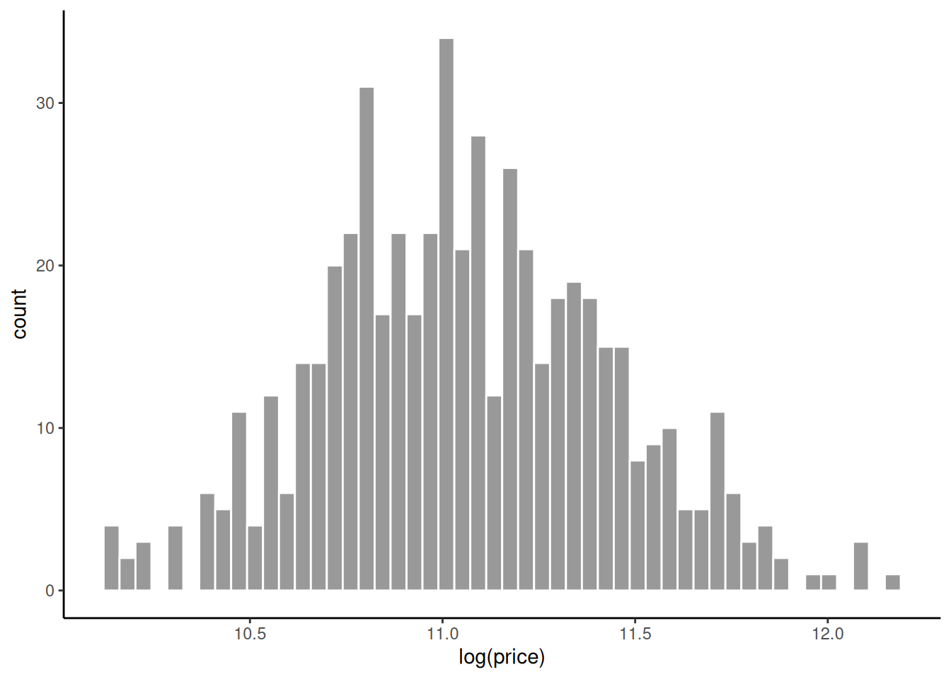
A very simple model of this data is that the logarithm of each of the \(n = 546\) house prices is drawn independently from a normal distribution with mean \(\mu\) and standard deviation of \(\sigma\): \[ \log(y_i) \sim N(\mu, \sigma), \quad \text{for $i \in 1 \ldots n$}, \] where \(y_i\) is the price of house \(i\). We can easily implement this model in R as follows:
M <- lm(log(price) ~ 1, data = housing_df)Let’s say we want to calculate the bootstrap confidence interval for the \(\sigma\) of this model. From any one lm model, we can obtain the estimate of \(\sigma\) using the function sigma(). To obtain the bootstrap confidence interval for \(\sigma\), we must bootstrap sample the housing_df data frame a relatively large number of times, with 10,000 samples being a quite typical number of samples. Using each bootstrap sample, we run the lm model above and then obtain our estimate of \(\sigma\) with the sigma() function. With 10,000 bootstrap samples, we then have 10,000 estimates of \(\sigma\), and we then calculate the 2.5th and 97.5th percentile of this distribution to obtain the 95% confidence interval of \(\sigma\).
There are a number of ways to perform this bootstrapping. Here, we will use base R’s sample function for the bootstrap sampling. Using this approach, we can draw a single bootstrap sample by sampling 546 rows, with replacement, from housing_df using code like the following:
n <- nrow(housing_df)
bootstrap_sample <- housing_df[sample(seq(n), replace = T),, drop = FALSE]
Extending this, a function to draw one bootstrap sample from any given data frame, execute an arbitrary lm model, and the return the estimate of \(\sigma\) in that model is as follows:
bootstrap_sigma <- function(formula, data_df) {
  n <- nrow(data_df)
  resampled_data <- data_df[sample(seq(n), replace = T),, drop = FALSE]
  M <- lm(formula, data = resampled_data)
  sigma(M)
}
We can use this with our model for the housing_df data as follows:
bootstrap_sigma(log(price) ~ 1, housing_df)[1] 0.3606936Of course, this will produce just one bootstrap estimate, so we need to repeat this line of code 10,000 times. This can be done in parallel. For that, we first start a new cluster of 4 workers.
the_cluster <- makeCluster(4)We then execute the bootstrap_sigma(...), as above, 10,000 times, distributing these function calls across the 4 workers. We can do this with, for example, the parLapply or parSapply commands that we used above. The results in both cases will be identical except that parLapply will return a list and parSapply will simplify this list to a vector. The latter case is preferable in this particular example, so we will use it here.
Were we to immediately try this, however, it would fail because the workers to do not have the function bootstrap_sigma nor the data housing_df. These are in the master process’s R environment. To copy bootstrap_sigma and housing_df to the workers we must do the following.
clusterExport(cl = the_cluster, varlist = c('bootstrap_sigma', 'housing_df'))Note that varlist is a vector of names, rather than the objects themselves.
Now, we can run the parSapply command.
bootstrap_estimates <- parSapply(the_cluster,
    seq(10000),
    function(i) bootstrap_sigma(log(price) ~ 1, data = housing_df)
)
The 95% confidence interval is obtained as follows:
boot_ci <- quantile(bootstrap_estimates, probs = c(0.025, 0.975))
boot_ci
2.5% 97.5%
0.3499309 0.3927598 The following plot shows the distribution of the estimates of \(\sigma\) and the lower and upper bounds of the 95% confidence interval.
tibble(estimates = bootstrap_estimates) %>%
  ggplot(aes(x = estimates)) +
  geom_histogram(bins = 50, col = 'white', fill = 'grey60') +
  geom_vline(xintercept = boot_ci[1], colour = 'red') +
  geom_vline(xintercept = boot_ci[2], colour = 'red')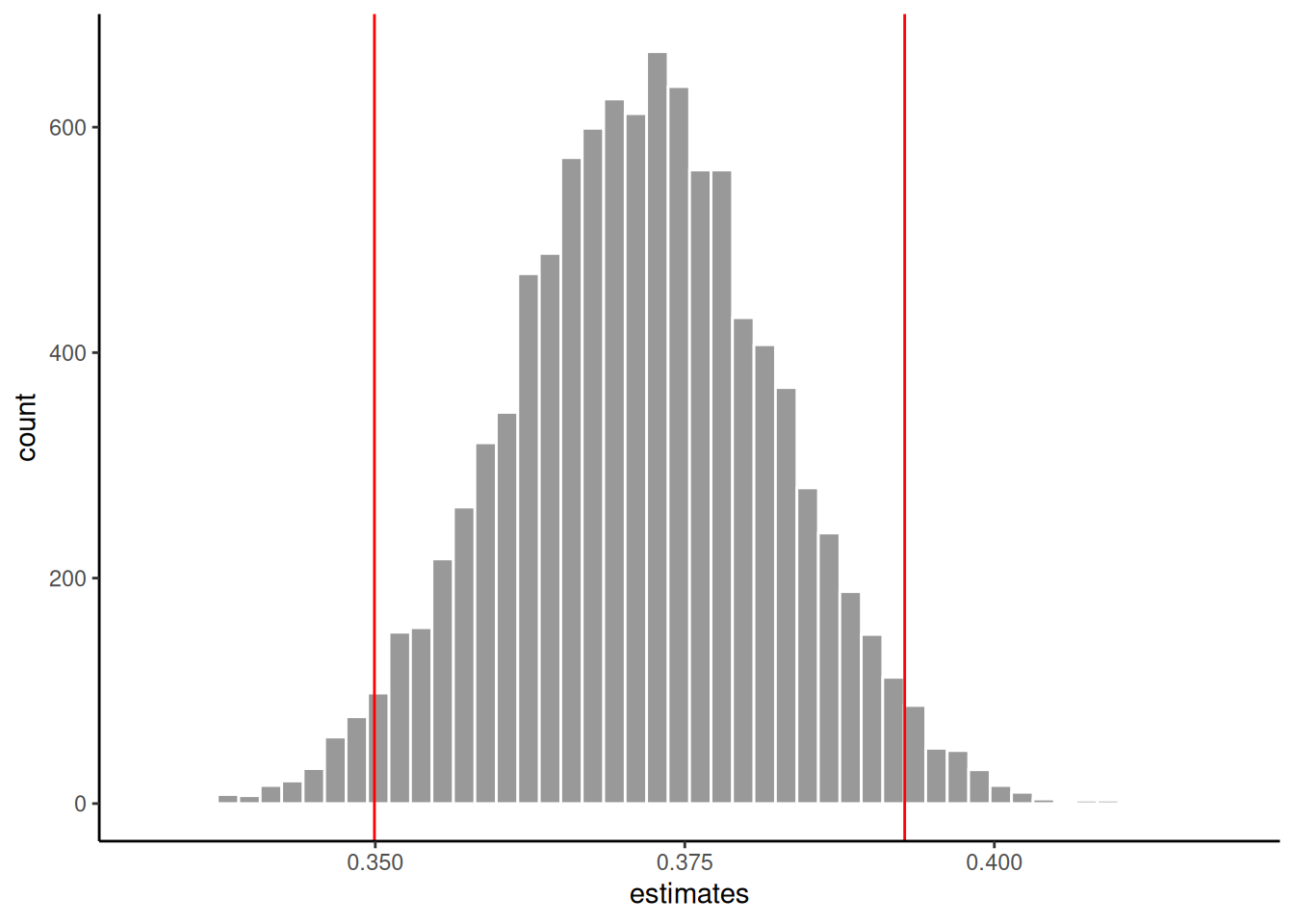
Let us now compare the time taken by parSapply to sample 10000 estimates and compare that to the time taken by sapply to do the same thing. For this timing, we will create two convenience functions, one for sapply and the other for parSapply:
sequential_bootstrap <- function(n){
  sapply(seq(n),
         function(i) {bootstrap_sigma(log(price) ~ 1, data = housing_df)}
  )
}

parallel_bootstrap <- function(n){
  parSapply(cl = the_cluster,
            seq(n),
            function(i) {bootstrap_sigma(log(price) ~ 1, data = housing_df)}
  )
}
We will use the relatively crude timing procedure of using Sys.time().
# parallel version with 4 workers
start_time <- Sys.time()
estimates <- parallel_bootstrap(10000)
parallel_version <- Sys.time() - start_time

# sequential version
start_time <- Sys.time()
estimates <- sequential_bootstrap(10000)
sequential_version <- Sys.time() - start_time
The times are as follows.
parallel_versionTime difference of 0.8289363 secssequential_versionTime difference of 3.021363 secsand so the parallel version is over 3.64 times as fast. However, it is interesting to note that this roughly linear speed up, which is the ideal speed up in parallel processing, is not always going to happen. Consider, for example, the case of obtaining just 5 bootstrap estimates.
# parallel version with 4 workers
start_time <- Sys.time()
estimates <- parallel_bootstrap(5)
parallel_version <- Sys.time() - start_time

# sequential version
start_time <- Sys.time()
estimates <- sequential_bootstrap(5)
sequential_version <- Sys.time() - start_time
The times are now as follows.
parallel_versionTime difference of 0.00445199 secssequential_versionTime difference of 0.003562927 secsand so the sequential version is actually faster. This occurs because there is overhead in farming out the tasks and communicating between the master and workers. For this reason, in general, it is always possible for a parallel processing task to be slower than its sequential counterpart.
stopCluster(the_cluster)Example 2: Parallel execution of multiple (multi-chain) MCMC models
In general, Markov Chain Monte Carlo (MCMC), which is used in statistics almost exclusively for inference in Bayesian models, is very computational intensive. In the MCMC based language Stan, and the brms R package that interfaces with Stan, we can easily execute the multiple MCMC chains within each model in parallel by just setting some options in the calling functions like brm or rstan. In other words, we can easily run the (typically 4) MCMC chains in a Stan model in parallel, and for anything other than a very small models, this usually gives us a speed up of approximately a factor of 4. However, in most real world analyses, we wish to perform multiple Stan models. When working on a high end workstation or cluster, we would like to take advantage of all the cores available to us to do this.
As an example, let us the affairs_df data set (the csv file of this data is here).
affairs_df <- read_csv('data/affairs.csv')This data gives us the number of extramarital affairs (affairs) in the last 12 months by each of 601 people. We could model this variable using, among other things, a Poisson, or negative binomial, or by the zero-inflated counterparts of these models. Likewise, we could use any combination of the eight predictor variables that we have available to us. Even though each model can use up to four cores, with one core being used per chain, if we were working on a workstation or cluster, we could execute many of these models simultaneously. For example, the workstation I am using now has 36 cores and so I could comfortably execute up to 8 models simultaneously, leaving a few cores free for other tasks. In principle, this could be accomplished by opening 8 different RStudio sessions and running a different model in each one, or running 8 different R scripts using Rscript in 8 Unix terminals. It is, however, much more convenient and manageable to have a single R script that creates 8 workers and farms out one of the 8 models to each one.
Let us consider the following Poisson regression model as a prototypical model.
M <- brm(affairs ~ gender + age + yearsmarried,
         data = affairs_df,
         cores  4,
         iter = 25000,
         family = poisson(link = 'log'))
Although not at all necessary for this model, we will use 25000 iterations per chain in order to resemble a larger and hence slower model. The running time, including the C++ compilation, for this model is approximately 48 seconds. Variants of this model might use either a different formula, or a different family or both. We can make a function that accepts different formulas and families. We do this, for reasons that will be soon clear, by creating a function that accepts one input argument that is a list with elements named formula and family.
affairs_model <- function(input){
  brm(input[['formula']],
      data = affairs_df,
      cores = 4,
      iter = 25000,
      family = input[['family']])
}
Now, we create a list of models specifications. Each element of this list is itself a list with two elements: formula and family. The formula is a brmsformula specifying the outcome variable and predictors. The family is one of the probability distribution families that brms accepts. Here, we specify six models, which are each combination of two sets of predictors and three different families.
model_specs <- list(

  # Poisson model with 3 predictors
  v1 = list(formula = brmsformula(affairs ~ gender + age + yearsmarried),
            family = poisson(link = 'log')),

  # Poisson model with 5 predictors
  v2 = list(formula = brmsformula(affairs ~ gender + age + yearsmarried + religiousness + rating),
            family = poisson(link = 'log')),

  # Negative binomial with 3 predictors
  v3 = list(formula = brmsformula(affairs ~ gender + age + yearsmarried),
            family = negbinomial(link = "log", link_shape = "log")),

  # Negative binomial with 5 predictors
  v4 = list(formula = brmsformula(affairs ~ gender + age + yearsmarried + religiousness + rating),
            family = negbinomial(link = "log", link_shape = "log")),

  # Zero-inflated Poisson with 3 predictors
  v5 = list(formula = brmsformula(affairs ~ gender + age + yearsmarried),
            family = zero_inflated_poisson(link = "log", link_zi = "logit")),

  # Zero-inflated Poisson with 3 predictors
  v6 = list(formula = brmsformula(affairs ~ gender + age + yearsmarried + religiousness + rating),
            family = zero_inflated_poisson(link = "log", link_zi = "logit"))

)
Using parLapply or a related function, we can farm each one of these model specification out to a worker. That worker will then compile the model and sample from it using four chains, with each chain on its own core. Thus, when sampling, \(6 \times 4\) cores will be in use. The 6 resulting models are then passed back to a list named results. First, we start the cluster of 6 workers, and to each, we export the affairs_df data frame. We also need to load the brms package on each worker, which we do with clusterEvalQ.
the_cluster <- makeCluster(6)

clusterExport(cl = the_cluster, varlist = 'affairs_df')
clusterEvalQ(cl = the_cluster, library("brms"))
We then run the parLapply using model_specs as the list and affairs_model as the function to which each element of the list will be applied. For comparison with the sequential model, we will time it.
start_time <- Sys.time()

results <- parLapply(cl = the_cluster,
                     model_specs,
                     affairs_model)

parallel_version <- Sys.time() - start_time
The running time is 80 seconds. For comparison, executing these models in a sequential functional like lapply could be done as follows.
start_time <- Sys.time()

sequential_results <- lapply(model_specs, affairs_model)

sequential_version <- Sys.time() - start_time
The running time in this case is 305 seconds, and so it is about 3.8 times slower than the parallel version.
Now, all the results of these models are in the list results with names v1, v2, etc. We can use these models completely as normal. For example, to extract the WAIC value of each model, we could create a helper function get_waic and apply it to each element by results.
get_waic <- function(model){
  waic(model)$estimates['waic', 'Estimate']
}
We will apply get_waic to results using a parallel functional like parLapply or parSapply, etc, but for these models, it could also be done using, for example, lapply or purrr::map.
waic_results <- parSapply(cl = the_cluster,
                          results,
                          get_waic)
waic_results v1 v2 v3 v4 v5 v6
3262.299 2910.228 1495.571 1471.391 1646.604 1617.808 stopCluster(the_cluster)Reuse
Citation
BibTeX citation:
@online{andrews2021,
  author = {Andrews, Mark},
  title = {Parallel Computing in {R} with the Parallel Package},
  date = {2021-07-07},
  url = {https://www.mjandrews.org/notes/rparallel/},
  langid = {en}
}
For attribution, please cite this work as:
Andrews, Mark. 2021. “Parallel Computing in R with the Parallel
Package.” July 7, 2021. https://www.mjandrews.org/notes/rparallel/.