Web scraping Wikipedia data tables into R data frames
web scraping
tidyverse
R
Wikipedia provides a lot of very useful tables of data. The data, however, are in the form of html tables, rather than some easy to import format like csv. To get this table into, for example, an R data frame requires some web scraping followed by data wrangling.
Wikipedia provides us with very large numbers of data tables. All of these tables, though perhaps with some exceptions, provide a detailed reference to the original sources of the data and, by virtue of being on a Wikipedia page, are free to use according tothe Creative Commons BY-SA 3.0 licence. However, if we want to do data analysis using R on data in these tables, we must first do some web scraping to extract the data from the html tables and then use dplyr and related tools to clean them up and convert them into a form that is easy to work with. Here, we provide a worked example of how to do this.
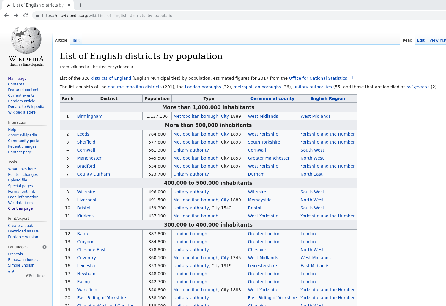
For this example, the page we will work with is List of English districts by population, and in particular the page version as of 28 January 2019 10:38 UTC.
Here’s a screenshot of that page where we see the main table:
We’ll need some R packages for web scraping, namely rvest, which provides a set of functions that are wrappers around functions in the httr and xml2 packages. We’ll then need dplyr for re-formatting and cleaning the data. We’ll use magrittr for some processing pipelines. We’ll use stringr for some renaming. We’ll use ggplot2 at the end for some visualizations.
library(tidyverse) # loads dplyr, ggplot2,
library(rvest)
library(magrittr)
library(stringr)
Web scraping the table
The web scraping is relatively painless. In addition to the url of the webpage, we also need to know the xpath node of the table in the page. This can be obtained using inspector tools in modern web-browsers, such as those provided by the DevTools in Chrome, see here. On the webpage used in this example, there’s actually just one html table, and we convert that to a tibble, although that final step is not strictly necessary.
webpage_url <- 'https://en.wikipedia.org/w/index.php?title=List_of_English_districts_by_population&oldid=879013307'

webpage_tables <-
  webpage_url %>%
  read_html() %>%
  html_nodes(xpath='//*[@id="mw-content-text"]/div/table') %>%
  html_table()

Df <- webpage_tables[[1]] %>%   # There's only one table
  as_tibble()
Data wrangling
Having read in the data into a data-frame, we now must do a series of typical dplyr data wrangling steps.
First, let’s take a look at the first 10 rows of the Df that we’ve obtained:
Df# A tibble: 338 × 6
Rank District Population Type `Ceremonial county` `English Region`
<chr> <chr> <chr> <chr> <chr> <chr>
1 More than 1,0… More th… More than… More… More than 1,000,00… More than 1,000…
2 1 Birming… 1,157,603 Metr… West Midlands West Midlands
3 More than 500… More th… More than… More… More than 500,000 … More than 500,0…
4 2 Leeds 822,483 Metr… West Yorkshire Yorkshire and t…
5 7 Sheffie… 566,242 Metr… South Yorkshire Yorkshire and t…
6 5 Cornwall 575,413 Unit… Cornwall South West
7 6 Manches… 568,996 Metr… Greater Manchester North West
8 9 Bradford 552,644 Metr… West Yorkshire Yorkshire and t…
9 10 County … 528,127 Unit… Durham North East
10 400,000 to 50… 400,000… 400,000 t… 400,… 400,000 to 500,000… 400,000 to 500,…
# ℹ 328 more rowsThere are a few things that need to be fixed:
- First, though this is maybe just a personal preference, we’ll convert column names to lower case and with no spaces.
- The original table’s sub-headers like
More than 1,000,000 inhabitants,More than 500,000 inhabitants, etc., have turned into rows with repeated values, and these need to be removed. - The population values need to be converted to integers.
- Some variables can be dropped to make a cleaner data frame.
To convert the column names, I’ll create a function using stringr and apply it using rename_with (see this blog post for more details on using rename_with):
tolower_no_spaces <- function(s){
  s %>%
    str_to_lower() %>%
    str_replace_all(' ', '_')
}

Df %<>% rename_with(tolower_no_spaces)
To deal with the inclusion of sub-headers rows, we need to filter out all rows that contain values like 250,000 to 300,000 inhabitants, Below 50,000, etc. If we just look at the rank variable, these cases can be relatively easily identified by whether they contain the words to, than or Below.
Df %>% filter(str_detect(rank, 'to|than|Below'))# A tibble: 12 × 6
rank district population type ceremonial_county english_region
<chr> <chr> <chr> <chr> <chr> <chr>
1 More than 1,000,0… More th… More than… More… More than 1,000,… More than 1,0…
2 More than 500,000… More th… More than… More… More than 500,00… More than 500…
3 400,000 to 500,00… 400,000… 400,000 t… 400,… 400,000 to 500,0… 400,000 to 50…
4 300,000 to 400,00… 300,000… 300,000 t… 300,… 300,000 to 400,0… 300,000 to 40…
5 250,000 to 300,00… 250,000… 250,000 t… 250,… 250,000 to 300,0… 250,000 to 30…
6 200,000 to 250,000 200,000… 200,000 t… 200,… 200,000 to 250,0… 200,000 to 25…
7 150,000 to 200,000 150,000… 150,000 t… 150,… 150,000 to 200,0… 150,000 to 20…
8 125,000 to 150,000 125,000… 125,000 t… 125,… 125,000 to 150,0… 125,000 to 15…
9 100,000 to 125,000 100,000… 100,000 t… 100,… 100,000 to 125,0… 100,000 to 12…
10 75,000 to 100,000 75,000 … 75,000 to… 75,0… 75,000 to 100,000 75,000 to 100…
11 50,000 to 75,000 50,000 … 50,000 to… 50,0… 50,000 to 75,000 50,000 to 75,…
12 Below 50,000 Below 5… Below 50,… Belo… Below 50,000 Below 50,000 That gives us an easy rule with which to filter them out:
Df %<>% filter(!str_detect(rank, 'to|than|Below')) We can now verify that the number of rows that we now have is the correct number, namely 326 (which is the current number of official districts that are in England).
nrow(Df)[1] 326Now, let’s take a look again at the first 10 rows:
Df# A tibble: 326 × 6
rank district population type ceremonial_county english_region
<chr> <chr> <chr> <chr> <chr> <chr>
1 1 Birmingham 1,157,603 Metropolitan… West Midlands West Midlands
2 2 Leeds 822,483 Metropolitan… West Yorkshire Yorkshire and…
3 7 Sheffield 566,242 Metropolitan… South Yorkshire Yorkshire and…
4 5 Cornwall 575,413 Unitary auth… Cornwall South West
5 6 Manchester 568,996 Metropolitan… Greater Manchest… North West
6 9 Bradford 552,644 Metropolitan… West Yorkshire Yorkshire and…
7 10 County Durham 528,127 Unitary auth… Durham North East
8 11 Wiltshire 515,885 Unitary auth… Wiltshire South West
9 12 Liverpool 496,770 Metropolitan… Merseyside North West
10 13 Bristol 479,024 Unitary auth… Bristol South West
# ℹ 316 more rowsNext, we’ll convert the population variable to an integer variable by first removing the commas in their values. However, before doing that, in the original permanent URL page, we notice that some values in the Population column have align="center" as values.
Df %>% filter(str_detect(population, 'align="center"'))# A tibble: 41 × 6
rank district population type ceremonial_county english_region
<chr> <chr> <chr> <chr> <chr> <chr>
1 "align=\"center\"" Northam… "align=\"… "Bor… Northamptonshire East Midlands
2 "align=\"center\"" Aylesbu… "align=\"… "" Buckinghamshire South East
3 "align=\"center\"" Bournem… "align=\"… "Uni… Dorset South West
4 "align=\"center\"" Wycombe "align=\"… "" Buckinghamshire South East
5 "align=\"center\"" South S… "align=\"… "" Somerset South West
6 "align=\"center\"" Harroga… "align=\"… "Bor… North Yorkshire Yorkshire and…
7 "align=\"center\"" Poole "align=\"… "Uni… Dorset South West
8 "align=\"center\"" Suffolk… "align=\"… "" Suffolk East of Engla…
9 "align=\"center\"" Sedgemo… "align=\"… "" Somerset South West
10 "align=\"center\"" Waveney "align=\"… "" Suffolk East of Engla…
# ℹ 31 more rowsThis is presumably just an typographic error. We could remove these rows, but when we convert to integers, population values in these rows will be converted to NA.
After we convert to integers, we’ll drop rank entirely because it can be calculated easily from population.
Df %<>% mutate(population = str_replace_all(population, ',', '') %>% as.integer()) %>%
  select(-rank)
Let’s look again at the first 10 rows:
Df# A tibble: 326 × 5
district population type ceremonial_county english_region
<chr> <int> <chr> <chr> <chr>
1 Birmingham 1157603 Metropolitan borou… West Midlands West Midlands
2 Leeds 822483 Metropolitan borou… West Yorkshire Yorkshire and…
3 Sheffield 566242 Metropolitan borou… South Yorkshire Yorkshire and…
4 Cornwall 575413 Unitary authority Cornwall South West
5 Manchester 568996 Metropolitan borou… Greater Manchest… North West
6 Bradford 552644 Metropolitan borou… West Yorkshire Yorkshire and…
7 County Durham 528127 Unitary authority Durham North East
8 Wiltshire 515885 Unitary authority Wiltshire South West
9 Liverpool 496770 Metropolitan borou… Merseyside North West
10 Bristol 479024 Unitary authority,… Bristol South West
# ℹ 316 more rowsThe type variable is quite inconsistent. The 326 English districts are in fact simply divided into 5 types but in our Df, the type variable is sometimes missing, or has values like “City (2012)” that do not correspond to one the five English district types, or has two pieces of information that are separated by a comma. Because of this overall inconsistency, we will drop the variable. However, it is possible to recover this information from joining this table with other tables of English districts such as from what is available on the List of English districts by area Wikipedia page.
Df %<>% select(-type) As a final fix, we can see that one district, namely Stockton-on-Tees, is listed as belonging to two regions of England:
Df %>% filter(district == "Stockton-on-Tees")# A tibble: 1 × 4
district population ceremonial_county english_region
<chr> <int> <chr> <chr>
1 Stockton-on-Tees 199966 Durham andNorth Yorkshire North East andYorkshire…Given that this district is listed here as part of North East England, we’ll change its listed region to North East.
Df %<>% mutate(english_region = recode(english_region,
                                       'North East andYorkshire and the Humber' = 'North East')
)
The final state of the data frame is now as follows:
Df# A tibble: 326 × 4
district population ceremonial_county english_region
<chr> <int> <chr> <chr>
1 Birmingham 1157603 West Midlands West Midlands
2 Leeds 822483 West Yorkshire Yorkshire and the Humber
3 Sheffield 566242 South Yorkshire Yorkshire and the Humber
4 Cornwall 575413 Cornwall South West
5 Manchester 568996 Greater Manchester North West
6 Bradford 552644 West Yorkshire Yorkshire and the Humber
7 County Durham 528127 Durham North East
8 Wiltshire 515885 Wiltshire South West
9 Liverpool 496770 Merseyside North West
10 Bristol 479024 Bristol South West
# ℹ 316 more rowsSummarizing and visualizing the data
Having extracted and cleaned the data, we can now obtain some summary statistics:
Df %>% summarize(number_of_districts = n(),
                 median_population = median(population, na.rm = T),
                 population_iqr = IQR(population, na.rm = T)
)
# A tibble: 1 × 3
number_of_districts median_population population_iqr
<int> <int> <dbl>
1 326 144593 120022And we can provide these summaries by English region too.
Df %>% group_by(english_region) %>%
  summarize(number_of_districts = n(),
            median_population = median(population, na.rm = T),
            population_iqr = IQR(population, na.rm = T)
  )
# A tibble: 9 × 4
english_region number_of_districts median_population population_iqr
<chr> <int> <dbl> <dbl>
1 East Midlands 40 111133 28106
2 East of England 48 141363 68772.
3 London 33 275887 107740
4 North East 10 205226. 139082.
5 North West 39 184728 162403
6 South East 66 131570. 49108.
7 South West 37 134230. 132337.
8 West Midlands 30 135008. 146617.
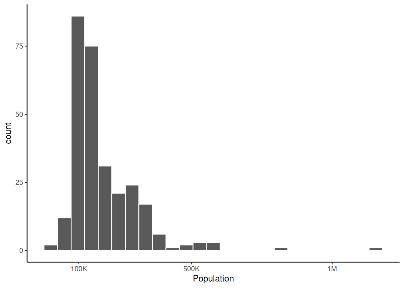
9 Yorkshire and the Humber 23 268603 181771.We can visualize the distributions of the population in each district.
ggplot(Df,
       aes(x = population)
) + geom_histogram(bins = 25, col='white') +
  theme_classic() +
  scale_x_continuous(name="Population",
                     breaks = c(10^5, 5*10^5, 10^6),
                     labels = c('100K', '500K', '1M')
        )
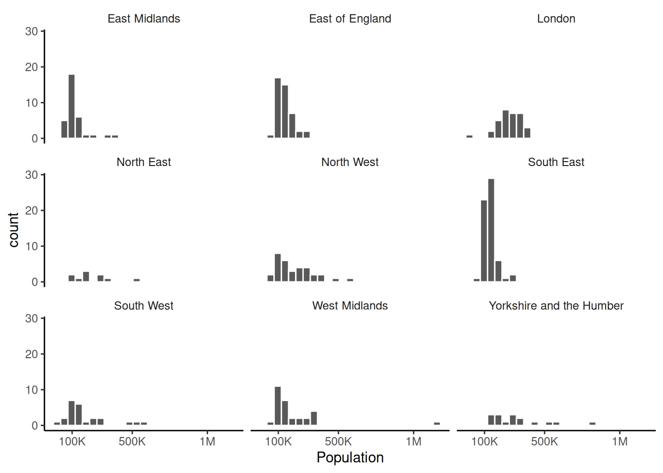
And do the same by region.
ggplot(Df,
       aes(x = population)
) + geom_histogram(bins = 25, col='white') +
  facet_wrap(~english_region)+  theme_classic() +
  theme(strip.background = element_blank()) +
  scale_x_continuous(name="Population",
                     breaks = c(10^5, 5*10^5, 10^6),
                     labels = c('100K', '500K', '1M')
  )
Reuse
Citation
BibTeX citation:
@online{andrews2019,
  author = {Andrews, Mark},
  title = {Web Scraping {Wikipedia} Data Tables into {R} Data Frames},
  date = {2019-01-28},
  url = {https://www.mjandrews.org/notes/scraping/},
  langid = {en}
}
For attribution, please cite this work as:
Andrews, Mark. 2019. “Web Scraping Wikipedia Data Tables into R
Data Frames.” January 28, 2019. https://www.mjandrews.org/notes/scraping/.