Statistical analysis of subgroups with nested data frames

Here, we will look at how to perform separate statistical analyses of each subgroup of a data set, the results of which can then be combined into a new data frame. For this, we will primarily use the nest, and related functions, in the tidyr package.

Many data sets, even relatively simple ones, can be seen as consisting of data subgroups. As a particularly simple example to illustrate this, consider the following data set:

library(tidyverse)

data_df <- tribble(
  ~x, ~y,
  'A', 1,
  'A', 7,
  'A', 11,
  'B', 3,
  'B', -7,
  'B', 5
)

The data_df data frame has two variables x and y. If we consider the values of x to indicate the group each observation belongs to, clearly data_df consists of two subgroups: those rows where x has the value of A, and those rows where x has the value of B.

Statistical models of data sets of this kind are very common practice. They include regression analyses with categorical predictor variables, but more generally, they involve multilevel (aka, hierarchical, or mixed-effects) modelling. Here, we will not discuss statistical modelling using, for example, multilevel models, but simply address ways of doing essentially exploratory data analysis of data sets like this. Specifically, we will look at how to efficiently perform separate statistical analyses of each subgroup of the data set and then combining their results into one new data frame. For this, we will primarily use the nest, and related functions, in the tidyr package.

The data set we will use in the examples below is named sleepstudy (csv file is here).

sleepstudy <- read_csv('data/sleepstudy.csv')
sleepstudy

# A tibble: 180 × 3
      rt   day subject
   <dbl> <dbl> <chr>  
 1  250.     0 s308   
 2  259.     1 s308   
 3  251.     2 s308   
 4  321.     3 s308   
 5  357.     4 s308   
 6  415.     5 s308   
 7  382.     6 s308   
 8  290.     7 s308   
 9  431.     8 s308   
10  466.     9 s308   
# ℹ 170 more rows

It consists of the average reaction times (rt) on each day without sleep (day) of a set of subjects (subject) in a sleep deprivation experiment. This data was originally obtained from the lme4 R package.

From group_by to group_by ... nest.

If we wanted to, for example, calculate the mean and standard deviation of the reaction time variable for each subject, the common tidyverse way to proceed would be to use a group_by operation followed by summary statistics calculation using summarise (or summarize):

sleepstudy %>% 
  group_by(subject) %>% 
  summarise(avg = mean(rt),
            stdev = sd(rt))

# A tibble: 18 × 3
   subject   avg stdev
   <chr>   <dbl> <dbl>
 1 s308     342.  79.8
 2 s309     215.  10.8
 3 s310     231.  21.9
 4 s330     303.  22.9
 5 s331     309.  27.2
 6 s332     307.  64.3
 7 s333     316.  30.1
 8 s334     295.  41.9
 9 s335     250.  13.8
10 s337     376.  59.6
11 s349     276.  42.9
12 s350     314.  63.4
13 s351     290.  29.0
14 s352     337.  47.6
15 s369     306.  37.5
16 s370     292.  59.2
17 s371     295.  36.5
18 s372     318.  35.8

While group_by and summarize are extremely generally useful, some subgroup analyses can not be performed this way. For example, consider the following plot of the data:

sleepstudy %>% 
  ggplot(aes(x = day, y = rt, colour = subject)) +
  geom_point(size = 0.5) +
  stat_smooth(method = 'lm', se = F) +
  facet_wrap(~subject) +
  theme_minimal() +
  theme(legend.position = 'none')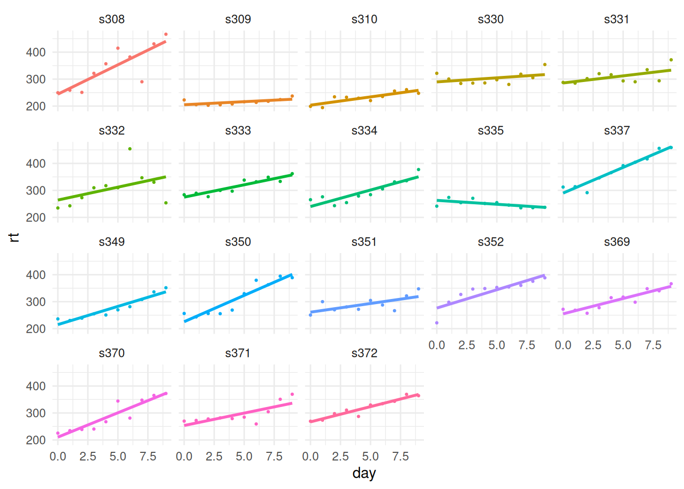

To produce this plot, ggplot performs a separate linear regression (using lm) using the data from each of the subjects. While it is undoubtedly useful that ggplot can produce this type of plot so easily, in some situations, we might wish to perform these lm models directly, not using ggplot, and save the resulting objects for further analysis. For example, we might wish to obtain a data frame that gives the \(R^2\) or the estimate of the residual standard deviation \(\hat{\sigma}\) for each subject. This can not be produced using group_by and summarize, but can be produced using group_by followed by a tidyr::nest operation, which produces a nested data frame on which further analyses can be performed.

To understand this, let us start by producing the nested data frame:

sleepstudy %>% 
  group_by(subject) %>% 
  nest()

# A tibble: 18 × 2
# Groups:   subject [18]
   subject data             
   <chr>   <list>           
 1 s308    <tibble [10 × 2]>
 2 s309    <tibble [10 × 2]>
 3 s310    <tibble [10 × 2]>
 4 s330    <tibble [10 × 2]>
 5 s331    <tibble [10 × 2]>
 6 s332    <tibble [10 × 2]>
 7 s333    <tibble [10 × 2]>
 8 s334    <tibble [10 × 2]>
 9 s335    <tibble [10 × 2]>
10 s337    <tibble [10 × 2]>
11 s349    <tibble [10 × 2]>
12 s350    <tibble [10 × 2]>
13 s351    <tibble [10 × 2]>
14 s352    <tibble [10 × 2]>
15 s369    <tibble [10 × 2]>
16 s370    <tibble [10 × 2]>
17 s371    <tibble [10 × 2]>
18 s372    <tibble [10 × 2]>

As we can see, we have produced a data frame with 18 rows, one for each subject, and with two columns. The first column indicates the subject’s identity. The second column is labelled data and we can see that it is list column, each element of which is a tibble data frame. Specifically, each element of the data list column is the data frame of the corresponding subject. For example, the first element of the data list column is the data frame corresponding to subject s308.

Now, if we want to perform a separate linear regression predicting rt from day for each subject, we can use a functional like purrr::map (see this blog post on functionals for details) to iterate over each separate data frame, passing it to an lm model. Each lm model will return an R object, which can then be saved in a new list column, which we may name model. This is done in the following code:

M_grouped <- sleepstudy %>% 
  group_by(subject) %>% 
  nest() %>% 
  mutate(
    model = map(data, ~lm(rt ~ day, data = .))
  )

M_grouped

# A tibble: 18 × 3
# Groups:   subject [18]
   subject data              model 
   <chr>   <list>            <list>
 1 s308    <tibble [10 × 2]> <lm>  
 2 s309    <tibble [10 × 2]> <lm>  
 3 s310    <tibble [10 × 2]> <lm>  
 4 s330    <tibble [10 × 2]> <lm>  
 5 s331    <tibble [10 × 2]> <lm>  
 6 s332    <tibble [10 × 2]> <lm>  
 7 s333    <tibble [10 × 2]> <lm>  
 8 s334    <tibble [10 × 2]> <lm>  
 9 s335    <tibble [10 × 2]> <lm>  
10 s337    <tibble [10 × 2]> <lm>  
11 s349    <tibble [10 × 2]> <lm>  
12 s350    <tibble [10 × 2]> <lm>  
13 s351    <tibble [10 × 2]> <lm>  
14 s352    <tibble [10 × 2]> <lm>  
15 s369    <tibble [10 × 2]> <lm>  
16 s370    <tibble [10 × 2]> <lm>  
17 s371    <tibble [10 × 2]> <lm>  
18 s372    <tibble [10 × 2]> <lm>  

Each element of the list column model is an lm R object where the lm formula was always rt ~ day and the data frame was the corresponding data frame in the data list column. So, for example, the first element of the model list column is the result of lm(rt ~ day) using the data of subject s308.

Unnesting

Let’s say we want to produce a new data frame that has two columns, subject and rsq, where rsq is the \(R^2\) estimate of the lm model for each subject. Note that if we have an lm model named M, then we can obtain the \(R^2\) estimate for M with summary(M)$r.sq. Using this, we extract the \(R^2\) from each subject’s lm model and put it in a vector column named rsq. We can do so using map_dbl, which returns a vector, and some standard dplyr operations, as follows:

M_grouped %>% 
  mutate(rsq = map_dbl(model, ~summary(.)$r.sq)) %>% 
  ungroup() %>% 
  select(subject, rsq)

# A tibble: 18 × 2
   subject   rsq
   <chr>   <dbl>
 1 s308    0.682
 2 s309    0.401
 3 s310    0.718
 4 s330    0.158
 5 s331    0.343
 6 s332    0.203
 7 s333    0.847
 8 s334    0.786
 9 s335    0.398
10 s337    0.933
11 s349    0.905
12 s350    0.869
13 s351    0.452
14 s352    0.745
15 s369    0.841
16 s370    0.853
17 s371    0.581
18 s372    0.912

Now, let’s say we want a data frame very similar to this but instead of just one new column, we want multiple new columns. For example, let’s say we want a column for each of \(R^2\), adjusted \(R^2\), the estimate of the residual standard deviation \(\hat{\sigma}\), and the estimates of the intercept and slope coefficients. For each of these quantities, we can extract the appropriate value from the lm model object using a function, and so we can create a function like the following that extracts all quantities and returns them as a vector:

model_summary <- function(M){
  c(rsq = summary(M)$r.sq,
    adj_rsq = summary(M)$adj.r.sq,
    sigma = sigma(M),
    intercept = unname(coef(M)[1]),
    slope = unname(coef(M)[2])
  )
}

We can see what this function will return for one of the models by extracting out one model from the model list column and passing it to model_summary:

M_grouped$model[[1]] %>% 
  model_summary()

        rsq     adj_rsq       sigma   intercept       slope 
  0.6815132   0.6417024  47.7796866 244.1926691  21.7647024 

We can not use this model_summary as the function inside a map_dbl, as we did above for the case of \(R^2\) alone, as map_dbl assumes that the value being returned by the function is a single value, rather than a vector. We can, however, use map as in the following code:

M_grouped %>% 
  mutate(summaries = map(model, model_summary))

# A tibble: 18 × 4
# Groups:   subject [18]
   subject data              model  summaries
   <chr>   <list>            <list> <list>   
 1 s308    <tibble [10 × 2]> <lm>   <dbl [5]>
 2 s309    <tibble [10 × 2]> <lm>   <dbl [5]>
 3 s310    <tibble [10 × 2]> <lm>   <dbl [5]>
 4 s330    <tibble [10 × 2]> <lm>   <dbl [5]>
 5 s331    <tibble [10 × 2]> <lm>   <dbl [5]>
 6 s332    <tibble [10 × 2]> <lm>   <dbl [5]>
 7 s333    <tibble [10 × 2]> <lm>   <dbl [5]>
 8 s334    <tibble [10 × 2]> <lm>   <dbl [5]>
 9 s335    <tibble [10 × 2]> <lm>   <dbl [5]>
10 s337    <tibble [10 × 2]> <lm>   <dbl [5]>
11 s349    <tibble [10 × 2]> <lm>   <dbl [5]>
12 s350    <tibble [10 × 2]> <lm>   <dbl [5]>
13 s351    <tibble [10 × 2]> <lm>   <dbl [5]>
14 s352    <tibble [10 × 2]> <lm>   <dbl [5]>
15 s369    <tibble [10 × 2]> <lm>   <dbl [5]>
16 s370    <tibble [10 × 2]> <lm>   <dbl [5]>
17 s371    <tibble [10 × 2]> <lm>   <dbl [5]>
18 s372    <tibble [10 × 2]> <lm>   <dbl [5]>

As we can see, summaries is list column where each element is vector of five values. We can now pivot, using something like a pivot_wider operation, these vectors to produce five new columns. We do this with an unnest_wider operation as follows:

M_grouped %>% 
  mutate(summaries = map(model, model_summary)) %>% 
  unnest_wider(col = summaries) %>% 
  ungroup() %>% 
  select(-c(data, model))

# A tibble: 18 × 6
   subject   rsq adj_rsq sigma intercept slope
   <chr>   <dbl>   <dbl> <dbl>     <dbl> <dbl>
 1 s308    0.682  0.642  47.8       244. 21.8 
 2 s309    0.401  0.326   8.87      205.  2.26
 3 s310    0.718  0.682  12.3       203.  6.11
 4 s330    0.158  0.0528 22.3       290.  3.01
 5 s331    0.343  0.260  23.4       286.  5.27
 6 s332    0.203  0.103  60.9       264.  9.57
 7 s333    0.847  0.828  12.5       275.  9.14
 8 s334    0.786  0.759  20.6       240. 12.3 
 9 s335    0.398  0.322  11.4       263. -2.88
10 s337    0.933  0.925  16.3       290. 19.0 
11 s349    0.905  0.893  14.0       215. 13.5 
12 s350    0.869  0.852  24.4       226. 19.5 
13 s351    0.452  0.383  22.8       261.  6.43
14 s352    0.745  0.713  25.5       276. 13.6 
15 s369    0.841  0.821  15.8       255. 11.3 
16 s370    0.853  0.834  24.1       210. 18.1 
17 s371    0.581  0.528  25.1       254.  9.19
18 s372    0.912  0.901  11.3       267. 11.3 

This procedure using nest and unnest_wider can therefore generally be used to produce data frames whose rows correspond to subgroups of the original data frame, and whose columns are the results of various statistical analyses performed separately on each subgroup.